The Big Picture
Penalizing only head-on (opposite-direction) crossings makes selfish agents settle into stable route choices, but finding the best global routing is generally NP-hard — practical algorithms work when a few structural parameters are small.
ON THIS PAGE
The Evidence
Modeling route interaction costs so only head-on encounters are penalized produces a game where pure-strategy stability is guaranteed and best-response moves converge in a bounded number of steps. A minimum-total-cost routing is always one of those stable outcomes, so the best-case selfish result matches the central planner’s best plan. On the flip side, finding that optimal plan is NP-complete in general, but several parameterized algorithms (fixed-parameter and XP) make optimal planning tractable for many realistic small-parameter cases. planning pattern
Not sure where to start?Get personalized recommendations
Data Highlights
1Best-response dynamics converge in at most w_max * k^2 * |E| steps (w_max = maximum edge weight, k = number of agents, |E| = number of edges).
2Price of Stability = 1 (a minimum-total-cost routing is always a Nash equilibrium), while the Price of Anarchy can be unbounded in worst cases.
3Centralized optimization is NP-complete in general, but the problem is fixed-parameter tractable when parameterized by vertex cover number plus the number of agents; reduction rules cap identical-node types to at most k representatives.
What This Means
Engineers planning decentralized route recommendations for robot fleets, warehouses, or vehicle lanes — because the model predicts when simple route advice yields stable behavior and when central planning is worth the cost. Technical leaders deciding whether to invest in centralized route optimization can use the parameterized results to know when those investments will pay off. Multi-Agent System
Key Figures
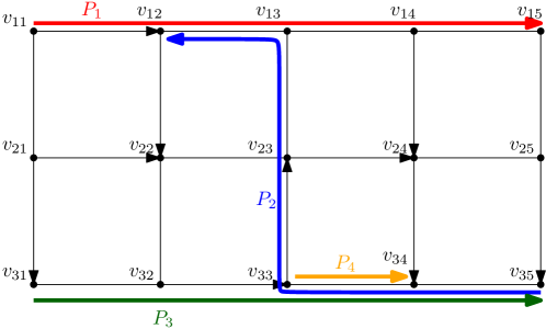
Fig 1: Figure 1: An example of CC-MAR. In this example, there are 4 agents with terminal pairs ( v 11 , v 15 ) (v_{11},v_{15}) , ( v 35 , v 12 ) (v_{35},v_{12}) , ( v 31 , v 35 ) (v_{31},v_{35}) , and ( v 33 , v 34 ) (v_{33},v_{34}) , respectively. The strategy of each agent is P i P_{i} for i ∈ { 1 , 2 , 3 , 4 } i\in\{1,2,3,4\} . Path P 1 P_{1} and path P 2 P_{2} cross each other on the edge { v 12 , v 13 } \{v_{12},v_{13}\} . Thus, the crossing cost between P 1 P_{1} and P 2 P_{2} is 1. The individual cost of agent 1 is also 1, as it has no other crossings. On the other hand, the individual cost of agent 2 is 4. This is because it crosses P 1 P_{1} on edge { v 12 , v 13 } \{v_{12},v_{13}\} , crosses P 3 P_{3} on edges { v 33 , v 34 } , { v 34 , v 35 } \{v_{33},v_{34}\},\{v_{34},v_{35}\} , and crosses P 4 P_{4} on edge { v 34 , v 35 } \{v_{34},v_{35}\} . The total cost of the strategy profile is the sum of all pairwise crossing costs, which is 1 ( from P 1 , P 2 ) + 2 ( from P 2 , P 3 ) + 1 ( from P 2 , P 4 ) = 4 1(\text{from }P_{1},P_{2})+2(\text{from }P_{2},P_{3})+1(\text{from }P_{2},P_{4})=4 .
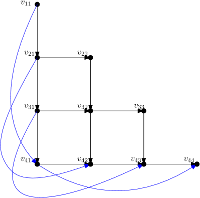
Fig 2: Figure 2: A grid-like graph when n = 4 n=4 . The blue arcs are threshold arcs.

Fig 3: Figure 3: The replacement of arc ( u , v ) (u,v) by a mixed u u - v v path consisting of ( u , u ′ ) , { u ′ , v ′ } , ( v ′ , v ) (u,u^{\prime}),\{u^{\prime},v^{\prime}\},(v^{\prime},v) .
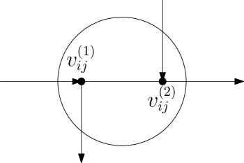
Fig 4: Figure 4: The resource gadget of r i j r_{ij} obtained by replacing vertex v i j v_{ij} .
Ready to evaluate your AI agents?
Learn how ReputAgent helps teams build trustworthy AI through systematic evaluation.
Learn MoreYes, But...
The model only charges opposite-direction (head-on) crossings and ignores delays or costs from same-direction crowding or timing, so it fits narrow corridors or one-lane scenarios best. Hardness results mean exact optimal routing is infeasible for large, general networks — the algorithms are practical when key structural parameters (like vertex cover or number of edges) are small. Some fixed-parameter results assume unweighted graphs or non-overlapping terminals, so check if your real network meets those constraints before applying them. State Inconsistency
Methodology & More
Introduce a routing model where agents pick source-to-destination paths and incur cost only when they traverse the same undirected edge in opposite directions. That asymmetric cost captures scenarios such as narrow corridors, one-lane roads, or robot aisles where same-direction flow is harmless but head-on encounters are costly. An aggregate cost sums pairwise crossing weights across edges. On the strategic side, the total crossing cost serves as a potential function, so selfish agents always admit a pure Nash equilibrium and best-response updates converge in at most w_max * k^2 * |E| steps (w_max is maximum edge weight). A minimum-total-cost profile is itself a Nash equilibrium (Price of Stability = 1), but worst-case selfish outcomes can be arbitrarily bad (unbounded Price of Anarchy). Computing a Nash equilibrium is polynomial when weights are polynomially bounded, but becomes hard (PLS-complete) otherwise. To connect to practical approach patterns, consider Consensus-Based Decision Pattern and Human-in-the-Loop Pattern. Human-in-the-Loop Pattern
Avoid common pitfallsLearn what failures to watch for
Credibility Assessment:
Authors include researchers with modest h-index (≈5); arXiv venue but nontrivial expertise signal.